Barnsley's fern

 

 

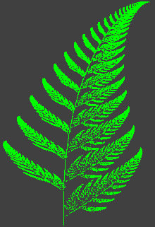Barnsley's fern is a fractal shape, discovered by Michael F. Barnsley at the Georgia Institute of Technology, that has many geometric features in common with a natural fern, most notably the appearance of frond-like forms at different scales. As in the case of real ferns, Barnsley's fern reveals smaller prominences along the edge of each frond that are miniature versions of the overall figure. Along these small prominences are still smaller protuberances, and so on. Barnsley's fern is created by the repetitive application of four relatively simple mathematical rules and is a type of fractal, introduced by Barnsley, known as an iterated function system (IFS).

 

Reference

1. Barnsley, Michael. Fractals Everywhere 2nd edition. San Francisco: Morgan Kaufmann, 1993.

 

Cantor dust

Cantor dust (Figure 1), also known as the Cantor set, is possibly the first pure fractal ever found – by Georg Cantor around 1872. To produce Cantor dust, start with a line segment, divide it in to three equal smaller segments, take out the middle one, and repeat this process indefinitely.

 

Although Cantor dust is riddled with infinitely many gaps, it still contains uncountably many points. It has a fractal dimension of log 2/log 3, or approximately 0.631.

 

Dragon curve

 

 

The Dragon curve is a classic example of a recursively-generated fractal shape. Benoit Mandelbrot called it the "Harter-Heighway" dragon curve and it formed the subject of one of Martin Gardner's Mathematical Games columns in Scientific American in 1967.¹ The Dragon curve fills out an "island" of positive area with a fractal boundary.

 

Reference

1. Gardner, Martin. Mathematical Magic Show: More Puzzles, Games, Diversions, Illusions and Other Mathematical Sleights-of-Mind from Scientific American. New York: Vintage, 1978.

 

fractal

A fractal is a geometric shape that can be subdivided at any scale into parts that are, at least approximately, reduced-size copies of the whole. The name "fractal," from the Latin fractus meaning a broken surface, was coined by Benoit Mandelbrot in 1975. The key property of fractals is self-similarity, which means that zooming in or zooming out of a fractal produces no overall change in appearance.

 

One of several technical definitions of a fractal is "a set of points whose topological dimension is less than its Hausdorff dimension". The topological dimension is an object's ordinary dimensionality – one in the case of a curve, two in the case of a surface, and so – and is always a whole number. The Hausdorff dimension, on the hand, measures how much space an object fills, and can take non-integer values if the object is very complex and twisty.

 

Some fractals show a strong regularity and rigid self-similarity and are produced by the repeated application of a set of rules that may be quite simple. Among the best known of these "iterated function" systems are the Koch snowflake, the Peano curves, the Sierpinski carpet, and the Sierpinski gasket. Other fractals, defined by a recurrence relation at each point in space, are among the most complex, beautiful, and beguiling mathematical structures known. They include the well-known Mandelbrot set and Lyapunov fractals. Finally, there are random fractals generated by stochastic rather than deterministic processes, for example fractal landscapes. Random fractals have the greatest practical use, and can be used to describe many highly irregular real-world objects, including clouds, mountains, coastlines and trees.

 

fractal dimension

A fractal dimension is a non-integer measure of the irregularity or complexity of a system; it is an extension of the notion of dimension found in Euclidean geometry. Knowing the fractal dimension helps one determine the degree of irregularity and pinpoint the number of variables that are key to determining the dynamics of the system.

 

Hausdorff dimension

A Hausdorff dimension, named after Felix Hausdorff, is a way to measure accurately the dimension of complicated sets such as fractals. The Hausdorff dimension coincides with the more familiar notion of dimension in the case of well-behaved sets. For example a straight line or an ordinary curve, such as a circle, has a Hausdorff dimension of 1; any countable set has a Hausdorff dimension of 0; and an n-dimensional Euclidean space has a Hausdorff dimension of n. But a Hausdorff dimension is not always a natural number. Think about a line that twists in such a complicated way that it starts to fill up the plane. Its Hausdorff dimension increases beyond 1 and takes on values that get closer and closer to 2. The same idea of ascribing a fractional dimension applies to a plane that contorts more and more in the third dimension: its Hausdorff dimension gets closer and closer to 3. As a specific example, the fractal known as the Sierpinski carpet has a Hausdorff dimension of just over 1.89.

 

Julia set

A Julia set is any of any infinite number of fractal sets of points on the complex plane (see Argand diagram) defined by a simple rule (Figure 2). Given two complex numbers z and c, and the recursion z_n+1 = z_n² + c, the Julia set for any given value of c, consists of all values of z for which z, when iterated in the equation above, does not "blow up" or tend to infinity. Julia sets are closely related to the Mandelbrot set, which is the set of all values of c for which z = 0 + 0i doesn't tend to infinity through application of the recursion. The Mandelbrot set is, in a way, an index of all Julia sets, For any point on the complex plane (which represents a value of c) a corresponding Julia set can be drawn. We can imagine a movie of a point moving about the complex plane with its corresponding Julia set. When the point lies inside the Mandelbrot set the corresponding Julia set is topologically unified or connected. As the point crosses the boundary of the Mandelbrot set, the Julia set explodes into a cloud of disconnected points called Fatou dust. If c is on the boundary of the Mandelbrot set, but not a waist point, the Julia set of c looks like the Mandelbrot set in sufficiently small neighborhoods of c.

 

Julia sets are named after the French mathematician Gaston Julia (1893–1978), whose most famous work, Memoire sur l'iteration des fonctions rationnelles, which provides the theory for Julia sets before computers were available to computer or represent them, was written in a hospital in 1918 at the age of twenty-five. As a soldier in World War I Julia had been severely wounded and lost his nose. He wrote his greatest treatise between the painful operations necessitated by his wounds.

 

Koch snowflake

The Koch snowflake is one of the most symmetric and easy to understand fractals. It is named after the Swedish mathematician Helge von Koch (1870–1924), who first described it in 1906.

 

To make the snowflake, start with a straight line and split it into three equal parts. Replace the middle part with two lines, both of the same length as the first three, creating a equilateral triangle missing the bottom line. The shape now consists of four straight lines with the same length. For each of these lines, repeat the process above, then continue the transformation indefinitely. The Koch curve has infinite length because each iteration increases the length of a line segment one third, and the iterations go on forever. The same kind of process can be applied to a tetrahedron. Take a regular tetrahedron (all side lengths the same) and glue to each of its faces a smaller regular tetrahedron (Each smaller tetrahedron is scaled down by a factor of ½ from the larger one, and placed on each face in an inverted fashion, so that it divides the face into four equilateral triangles and covers the center one.) Then iterate this process. Intuition suggests that the end product might be a very strange-looking jagged object. But in fact, in the limit, as the number of iterations tends to infinity, the result is a perfect cube! The cube has side length t/√2, where t is the length of one of the edges of the regular tetrahedron you started with.

 

Variations on the flat Koch snowflake include the so-called exterior snowflake, the Koch antisnowflake, and the flowsnake curves.

 

L-system

An L-system is a method of constructing a fractal that is also a model for plant growth. L-systems use an axiom as a starting string and iteratively apply a set of parallel string substitution rules to yield one long string that can be used as instructions for drawing the fractal. Many fractals, including Cantor dust, the Koch snowflake, and the Peano curve, can be expressed as an L-system.

 

Lyapunov fractal

 

 

The Lyapunov fractal is a particularly photogenic type of fractal that is popular with computer artists. It also represents a simple biological model of population growth in which the degree of the growth of the population can periodically alter between two values a and b.

 

Mandelbrot set

The Mandelbrot set is the best known fractal and one of the most complex and beautiful mathematical objects known. It was discovered by Benoît Mandelbrot in 1980 and named after him by Adrien Douady and J. Hubbard in 1982.

 

The Mandelbrot set is produced by the incredibly simple iteration formula:

 

    z_n+1 = z_n² + c,

 

where z and c are complex numbers and z₀ = 0. This can be written without complex numbers as

 

    x_n+1 = x_n² - y_n² + a, and
    y_n+1 = 2x_ny_n + b

 

where z = (x, y) and c = (a, b). The Mandelbrot set consists of all the points on the complex plane for which the function z² + c doesn't diverge under iteration (Fig 4).

 

A computer is essential for carrying out the necessary calculations and for producing pictures of this remarkable structure. For the purposes of computation, the complex plane is broken down into pixels (picture elements), the coordinates of each of which supply the constant c in z² + c. For each pixel (value of c) the function is iterated. If the function either rapidly diverges (blows up) or rapidly converges (collapses), the pixel is left black. If the function is more indecisive about which way it is heading, it is allowed to iterate longer. In some cases the iterations could go on for a very long time before it became clear that the function would ultimately diverge, so a limit is established, known as the depth, beyond which iterations are stopped. If the depth is reached without divergence, the corresponding pixel is left black as though it were in the set. At locations where divergence is indicated prior to hitting the limit, the pixel is displayed according to a scale that represents how many iterations are needed to show divergence.

 

The whole Mandelbrot set lies within a circle of radius 2.5 centered at the origin of the complex plane. Although finite in area, the Set has a boundary that is infinitely long and has a Hausdorff dimension of 2. The overall appearance of the Mandelbrot set is that of a series of disks. These disks have irregular borders and decrease in size heading out along the negative real axis; moreover, the ratio of the diameter of one disk to the next approaches a constant. More complex shapes branch out from the disks. One region of the Mandelbrot set containing spiral shapes is known as Seahorse Valley because it resembles a seahorse's tail. A computer can be used, like a microscope, to zoom in on different parts of the set. This reveals that, although the shape is infinitely complex, it also displays self-similarity with regions that look like the outline of the entire set.

 

The Mandelbrot set also exhibits symmetry on different levels. It is identically symmetrical about the real axis, and almost symmetrical at smaller scales. This kind of "near-but-not-quite" symmetry is one of the most unexpected properties to find in an object generated from such a simple formula and process. The Mandelbrot set was created by Mandelbrot as an index to the Julia sets. Each point in the complex plane corresponds to a different Julia set, and those points within the Mandelbrot set correspond precisely to the connected Julia sets.

 

Menger sponge

 

 

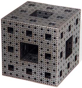The Menger sponge is a famous fractal solid that is the three-dimensional equivalent of the Sierpinski carpet (which, in turn, is the one-dimensional equivalent of Cantor dust). To make a Menger sponge, take a cube, divide it into 27 (= 3 × 3 × 3) smaller cubes of the same size and remove the cube in the center and the six cubes that share faces with it. What's left are the eight small corner cubes and twelve small edge cubes holding them together. Now, imagine repeating this process on each of the remaining 20 cubes. Repeat it again. And again ... ad infinitum. The Menger sponge was invented in 1926 by the Austrian mathematician Karl Menger (1902–1985).

 

pathological curve

A pathological curve is a curve often specifically devised to show the falseness of certain intuitive concepts. In particular, the image of continuity as a smooth curve in our mind's eye severely misrepresents the situation and is the result of a bias stemming from an overexposure to the much smaller class of differentiable functions. A chief lesson of pathological curves is that continuity is a weaker notion than differentiability. Many pathological curves are fractals, such as Cantor dust, including space-filling curves, such as the Peano curve. The earliest known example is the graph of Weierstrass' non-differentiable function.

 

Peano curve

The Peano curve is the first known example of a space-filling curve (Figure 5). Discovered by Giuseppe Peano in 1890, its effect was like that of an earthquake on the traditional structure of mathematics. Commenting in 1965 on the impact of the curve in Peano's day, N. Ya Vilenkin said: "Everything has come unstrung! It's difficult to put into words the effect that Peano's result had on the mathematical world. It seemed that everything was in ruins, that all the basic mathematical concepts had lost their meaning."

 

Today, the Peano curve is recognized as just one of an infinite class of familiar objects known as fractals. But at the end of the nineteenthth century it was an extravagant, completely counterintuitive thing; indeed, it was something that had been believed impossible. Writing of Peano's result in Grundzüge der Mengenlehre in 1914, Felix Hausdorff said: "This is one of the most remarkable facts of set theory."

 

Originally, the Peano curve was derived purely analytically, without any kind of drawing or attempt at visualization. But the first few steps in drawing it, as shown in the diagrams, are easy enough, even though the finished product is unattainable in this way – and totally unimaginable. To fill the unit square, as the Peano curve does, without leaving any holes, the curve has to be both continuous and self-intersecting.

 

Sierpinski carpet

 

 

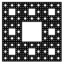The Sierpinski carpet is a fractal, named after Waclaw Sierpinski, that is derived from a square by cutting it into nine equal squares with a 3 × 3 grid, removing the central piece, and then applying the same procedure ad infinitum to the remaining eight squares. It is one of two generalizations of the Cantor set to two dimensions; the other is the Cantor dust. The carpet's Hausdorff dimension is log 8/log 3 = 1.8928...

 

Sierpinski gasket

The Sierpinski gasket is a fractal, also known as the Sierpinski triangle or Sierpinski sieve, produced by the following set of rules:

 

1. Start with any triangle in a plane.
2. Shrink the triangle by ½, make three copies, and translate them so that each triangle touches the two other triangles at a corner.
3. Repeat step 2 ad infinitum.

 

The gasket can also be made by starting with Pascal's triangle, then coloring the even numbers white and the odd numbers black. Most curiously, it can be generated by a game of chance. Start with three points, labeled 1, 2, and 3, and any starting point, S. Then select randomly 1, 2, or 3, using a die or some other method. Each random number defines a new point halfway between the latest point and the labeled point that the random number indicates. When the game has gone on long enough the pattern produced is the Sierpinski gasket.

 

The gasket has a Hausdorff dimension of log 3/log 2 = 1.585..., which follows from the fact that it is a union of three copies of itself, each scaled by a factor of ½. Adding rounded corners to the defining curve gives a non-intersecting curve that traverses the gasket from one corner to another and which Benoit Mandelbrot called the Sierpinski arrowhead.

 

space-filling curve

A space-filling curve is a curve that passes through every point of a finite region (such as a unit square or unit cube) of a n-dimensional space, where n is greater than or equal to 2. A well-known example is the Peano curve.

 

Weierstrass nondifferentiable function

The Weierstrass nondifferentiable function is the earliest known example of a pathological function – a function that gives rise to a pathological curve. It was investigated by Weierstrass but had been first discovered by Bernhard Riemann, and is defined as:

 

   

 

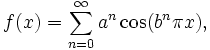
where 0 < a < 1, b is a positive odd integer, and ab > 1 + 3π/2.

 

The Weierstrass function is everywhere continuous but nowhere differentiable; in other words, no tangent exists to its curve at any point. Constructed from an infinite sum of trigonometric functions, it is the densely-nested oscillating structure that makes the definition of a tangent line impossible.