calculus
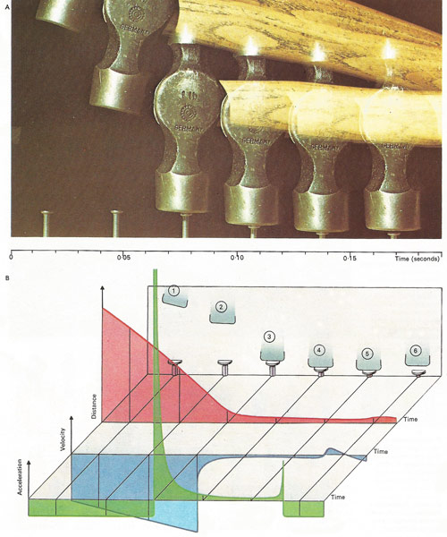
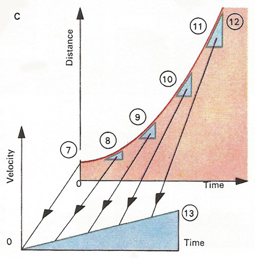
A falling hammer is shown [A] in six exposures 0.03 s apart and the hammer position curve [D in diagram B] follows them [1-6]. Its changing slope is important and diagram C explains how this is measured, like a road gradient, by tangent triangles with so many units vertically for each one horizontally. The slopes at points 7-11 of line 12 are 0:2, 1:2, 2:2, 3:2 and 4:2 respectively - or 0, 1/2, 1, 1 1/2 and 2. Line 13 plots the increasing slope of line 12. (Obtaining a slope curve from a curve is called differentiation; the reverse in integration.) In [B], the slope of the distance curve for the first exposure is given by a vertical drop of 2.8 cm for a time interval, measured horizontally, of 0.02 s. So the velocity here is 2.8 cm in 0.02 s = 140 cm/s. Similar slope measurements give the velocity at other points and yield velocity curve V which initially increases downwards, like the distance. The acceleration (the rate of change of velocity with time) is the slope of the velocity curve - constant while the hammer is falling freely (curve A). At exposure 3, the hammer hits the nail at 200 cm/s and things start to happen. In a millisecond (thousandth of a second) the velocity is braked back to about 40 cm/s (curve V); this rapid deceleration drives A off-scale upwards to perhaps 100 times its free-fall value. Newton's law then gives a correspondingly large force on the nail, 100 times the weight of the hammer, and this is how the hammer works - driven by the force generated by rapid deceleration of the head. As the wood seizes the nail the shock kicks the hammer upwards; then in free fall again the hammer resumes steadily increasing downward velocity and constant acceleration.
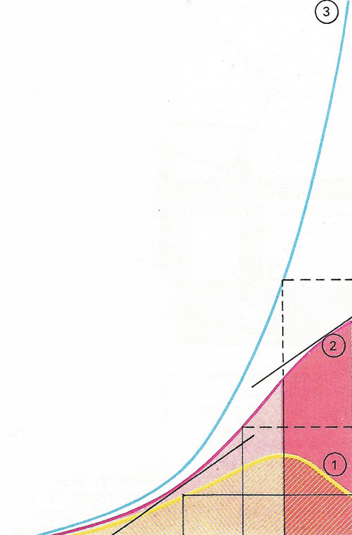
Calculus can be used to analyze a headline such as: "Government acts to hold prices; rate of increase of inflation cut back". Suppose curve 1 is the rate of increase of inflation. Inflation itself will be the integral of 1 - curve 2, whose rate if increase at each point is proportional to the height of curve 1. Thus the slopes shown (black) are equal. Inflation is the rate of increase of prices, so prices (curve 3) are the integral of curve 2. It is then obvious that prices are not being "held".
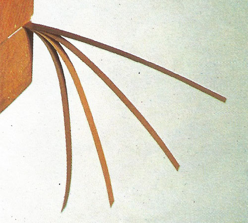
The curvature of a beam at any point depends on its loading. A projecting strip is bent at each point by the weight of the length beyond it and calculus-based beam-theory adds up all these changing curvatures to arrive at the final shape of self-loaded beams. These plastic strips have different thicknesses and their degrees of deflection vary roughly as the inverse square of their thickness. Engineering beams do not sag as much but the same design principles apply.
![The cost benefit of increased insulation on a pipe [A] depends on reduction of heat loss (E on the pale blue) offsetting higher capital costs C.](../../images3/cost_benefit_analysis.jpg)
The cost benefit of increased insulation on a pipe [A] depends on reduction of heat loss (E on the pale blue) offsetting higher capital costs C. Their sum is least at MI. Increasing diameter reduces pumping costs (E on the dark blue) while raising capital cost (least at MD). The overall minimum cost is (MI1, MD1) at X. A chemical plant [B] must minimize cost over hundreds of variables.
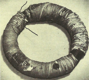
Faraday's "anchor ring" was the first-ever transformer. It revealed the law that the voltage on the output coil depends on the rate of change of voltage on the input coil.
Calculus is the branch of mathematics that deals with (1) the rate of change of quantities (which can be interpreted as the slopes of curves), known as differential calculus, and (2) the length, area, and volume of objects, known as integral calculus. It can be seen as an extension of analytical geometry.
Calculus was one of the most important developments in mathematics and also in physics, much of which involves studying how quickly one quantity changes with respect to another. It is no coincidence that one of the founders of calculus was the English physicist and mathematician Isaac Newton (1642–1727); another was the German mathematician and philosopher Gottfried Leibniz (1646–1716).
Leibniz published his research in the journal Acta Eruditorum in 1684 and Newton in his treatise Principia in 1687, though Newton actually began work on the theory first. Their new mathematical system attempted to calculate motion and change. However, the two variants described change differently. For Newton, change was a variable quantity over time; for Leibniz it was the difference ranging over a sequence of infinitely close values.
William Fogg Osgood (1864–1943) said: "The calculus is the greatest aid we have to the application of physical truth in the broadest sense of the word." Although students nowadays learn the differential calculus first, the integral calculus has older roots.
Introduction
In a "political vocabulary" complied for the daily newspaper the Guardian, the noun "decrease" was cynically defined as: "reduction in rate of increase – as in unemployment, crime, inflation, taxation, etc". This not only exposes official double-talk but also highlights the universality of a central concept of calculus – rate of change.
Rates of change became important in physics in 1638 when Galileo (1564–1642) concluded that a falling or thrown body had a downward velocity that increases steadily – that is, its rate of increase of downward velocity is constant. What then is its trajectory? It took the genius of Newton and Leibniz to solve this problem neatly and completely; the tool they created for the job was calculus.
Velocity, said Newton, is rate of change of position with time – 60km/h, for instance. Similarly, acceleration is rate of change of velocity with time. A car that takes three seconds to reach a speed of 60km/h from a standing start has an average acceleration of 20km/h per second. Galileo's law is that the downward acceleration of a falling body is constant. Calculus provides the methods of obtaining velocity from acceleration and position from velocity, and the whole problem is neatly solved. The calculus operation of deriving velocity from position, for example, is called differentiation. Its inverse is called integration.
The simplicity in symbolism
All mathematics is a sort of symbolic machinery for making subtle conceptual deductions without having to think them out – all the thought has been built into symbolism. Long division, for example, enables 431,613 to be divided by 357 by the unthinking application of a few rules; it is not necessary to know why it works, or what division really means. Calculus is perhaps the supreme example of a symbolism whose economical elegance reduces intractably complex and elusive problems to back-of-an-envelope simplicity.
In mechanics, the branch of physics for which calculus was invented, it is omnipresent in Newton's second law of motion: force equals mass multiplied by acceleration. Given any two of these quantities, the equation defines the third. Consider an internal combustion engine. What is he instantaneous acceleration of the piston as the crank passes top dead center? Calculus provides the answer so that, knowing the piston's mass, it is possible to find the force on it that must be withstood by the connecting-rod. For what speed will this force become excessive? Again, the pressure on the piston during the power stroke is changing every instant with the burning of the charge and the changing volume of the gasses in the cylinder as the piston descends. What then is the total energy imparted to the piston by the whole stroke and for what moment of ignition is it a maximum? This and a myriad of other mechanical problems could hardly be formulated, let alone solved, without calculus.
Electronic applications
One powerful application of calculus is in seeking maxima, minima, and optima generally. A vertically thrown ball is momentarily stationary at the top of its flight: when the height with time is zero. It can be found by differentiating the expression relating height and time and putting this equal to zero. This is a general rule of great value – for all technology is governed by the search for optima.
What is the optimum speed for a journey, for example? Too slow wastes time, too fast wastes fuel; both of these have an assignable cost. Calculus enables the rate of change of overall cost with speed to be found and the speed of which it is zero. This must then be the speed for minimum cost. Such calculations are essential in making the best use of ships and aircraft and the same principles apply in all searches for the best design or flow-rate or working temperature of almost every industrial system.
Universal principle
Many physical laws embody the same principle. Thus light traverses an optical system by a path that takes less time than any other possible path - a principle from which the whole of classical optics can be derived. Indeed Leibniz, possibly carried away by the power of his creation, proposed that the whole universe had been designed in some such mighty self-optimization process and that this was the best of all possible worlds. He seems not to have considered the possibility that it might be the worst.
Differential calculus
Consider the function y = f(x). This may be plotted as a curve on a set of Cartesian coordinates. Assuming that the curve is not a straight line, tangents to it at different points will have different gradients. Two points close together on the curve, (x, y) and (x+δx, y + δy), where δx and δy mean very small distances in the x- and y-directions, will usually have tangents of similar, though not identical, gradients. The gradient of the line passing through these two points is given by
[(y + δy) - y]/[(x + δx) - x],
and is the same as that of a tangent to the curve somewhere between the two points. The smaller δx is, the closer the two gradients will be; and if δx is infinitely small, they will be identical. This limit as x → 0 is the derivative
dy/dx or f '(x)
of the function and is given by (putting f(x) in place of y):
f'(x) = lim (δx→0) [f(x + δx) - f(x)] / δx.
This formula will give the gradient of the curve for f(x) at any value of x. For example, in the parabola y = x 2 the derivative at x = a is given by
f '(a) = lim (x→a) (x 2 - a2)/(x - a)
= lim (x→a) (x + a)(x - a)/(x - a)
= lim (x→a) (x + a) = 2a.
Hence we can say that f '(x) = 2x for f(x) = x 2. This process is termed differentiation. In general if f(x) = x 2 then
f '(x) = z.xz - 1, and the second derivative
f ''(x) or d 2x/dx 2,
the result of differentiating again, is (z - 1).z.x z - 2, and so on.
Integral calculus
The derivative of f (x) gives the instantaneous rate of change of f(x) for a particular value of x. Now, consider the plot of y = f '(x), and assume that f '(x) = f(x) = 0 when x = 0. A very thin strip with one vertical side the f '(x)-axis and the other the line joining the points (δx, 0) and (δx, f '(δx)), will have an area of approximately δx, f '(δx). A second thin strip drawn next to it will have an area of roughly δx, f '(2δx), and so on. The area between the curve and the x-axis from x = 0 to x = a will therefore be roughly δx.f '(δx) + δx.f '(2δx) + ... + δx.f '(a + δx) + δx.f '(a). If one plots on a different graph x against (area of strip 1), (area of strips 1 + 2), area of strips 1 + 2 + 3), etc., one finds that one is plotting a close approximation to y = f(x). This reverse of differentiation is called integration, and f (x) is the integral of f '(x). We find, too, that the integral of x z is
x z + 1 / (z + 1)
which is what one would expect. This is the indefinite integral of x z since we have not specified how much of the curve we wish to consider, and we must add a constant, c, since the derivative of any constant is 0. As integration is the sum of the areas of the strips described, we symbolize it by an extended S. For example, the integral from 0 to 1 of x 2 is written as
x 2.dx.
Calculus of variations
The calculus of variations is an extension of calculus concerned with the examination of definite integrals and the calculation of their maximization and minimum values. One of its most famous problems was the brachistochrone problem, in which it was required to find out the least time taken for a particle to fall, under the influence of gravity alone, between two points at different heights though not vertically above each other. The path is in fact a cycloid, the solution involving minimization of the integral that expresses the path. An example of a problem involving calculus of variations is to find the shape of a cable suspended from both ends (see catenary).