analytical geometry
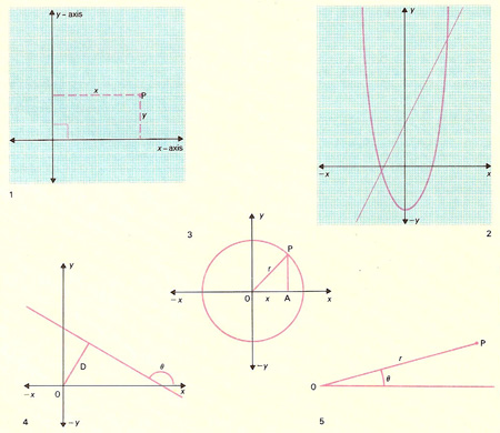
(1) Cartesian coordinate system whose origin is at O where the x- and y-axes intersect at right angles. The position of a point P is determined by its coordinates (x, y). (2) On this coordinate system, the set of all points that satisfy a particular relationship between x and y may be plotted. Here the set of all points satisfying the equation y = 2x + 3 forms a straight line cutting the y-axis at y = 3 and the x-axis at –1½. The set of all points satisfying y = x 2 + 3 forms a parabola cutting the y-axis at y = –3 and x = +√3 and x = –√3. Note the symmetry of the curve about the y-axis. (3) Again using these axes we can find the equation for the set of all points lying on the circumference of a circle. Here the circle has radius r, and its center lies at the origin O. Applying Pythagoras' theorem, we see that for any point P on the circumference, x 2 + y 2 = r 2. This relationship is the equation of the circle. (4) A straight line may be determined using line coordinates, where the angle θ that the line makes with the x-axis and the perpendicular distance D from the line to the origin are specified. (5) Polar coordinates employ the distance r of a point P from the origin O and the angle θ which the line OP makes with a fixed line called the polar axis. The coordinates of P are therefore (r, θ).
Analytical geometry, also known as coordinate geometry or Cartesian geometry, is the type of geometry that describes points, lines, and shapes in terms of coordinates, and that uses algebra to prove things about these objects by considering their coordinates.
René Descartes laid down the foundations for analytical geometry in 1637 in his Discourse on the Method of Rightly Conducting the Reason in the Search for Truth in the Sciences, commonly referred to as Discourse on Method. This work provided the basis for the calculus, which was introduced later by Isaac Newton and Gottfried Leibniz.
Plane geometry
In plane geometry, there are usually two axes, commonly designated the x- and y-axes, at right angles. The position of a point in the plane of the axes may then be defined by a pair of numbers (x, y), its coordinates, which give its distance in units in the x- and y-direction from the origin (the point of intersection) of the two axes. In three dimensions there are three axes, usually at mutual right angles, commonly designated the x-, y-, and z-axes.
In the coordinates (x, y, z), consider the situation when two of these have fixed values: there is a set of points, called a coordinate line, corresponding to all values of the third coordinate. Repeating this for each of the three coordinates, it can be seen that through each point defined by this coordinate system there are three coordinate lines. For all points, all three of these are straight (the system is rectilinear) and at mutual right angles (the system is rectangular).
In plane polar coordinates there are two coordinated lines through each point: these are at right angles and one is curved (the system is rectangular and curvilinear).
Equation of a curve
A curve may be defined as a set of points. A relationship may be established between the coordinates of every point of the set, and this relationship is known as the equation of the curve. The simplest form of plane curve is the straight line, which in the system we have described has an equation of the form y = ax + b, where a and b are constants. Set a = 2 and b = 3: then, if x = 1, y = 2 + 3 = 5, if x = 2, y = 7, and so on; and conversely if y = 1, x = (1 – 3)/2 = –1, and so on. All points whose coordinates satisfy the relationship y = 2x + 3 will lie on this line.
Equations of curves may involve higher powers of x or y: a parabola may be expressed as y = ax 2 + b.